Computer Architecture

Table Of Contents

• Chapter 1
  • 1.1 Introduction
  • 1.2 Classes of Computers
    • Flynn’s Taxonomy of Computer Architectures:
  • 1.3 Defining Computer Architecture
  • 1.4 Trends in Technology
  • 1.9 Quantitative Principles of Computer Design
  • Summary
• Chapter 2: Memory Hierarchy Design
  • 2.1 Introduction
  • Appendix B
    • Physical CPU Layout V1
    • Virtual Memory

Bookmark

Stopped reading at page: 76 -> Appendix B-4

Chapter 1

1.1 Introduction

RISC (Reduced Instruction Set Computer) enabled by C and UNIX/LINUX focused on two performance techniques:

1. ILP (Instruction level parallelism)
2. Caches

Intel x86 (80x86) → CISC (with internal RISC-like execution)
ARM → Pure RISC

1.2 Classes of Computers

Hard real-time system has absolute deadlines, and if those allotted time spans are missed, a system failure will occur.
In soft real-time systems, the system continues to function even if missing a deadline, but with undesirable lower quality of output.

There are basically two kinds of parallelism in applications:

1. Data-Level Parallelism (DLP) arises because there are many data items that can be operated on at the same time.
2. Task-Level Parallelism (TLP) arises because tasks of work are created that can operate independently and largely in parallel.

Computer hardware in turn can exploit these two kinds of application parallelism in four major ways:

1. Instruction-Level Parallelism exploits data-level parallelism at modest levels with compiler help using ideas like pipelining and at medium levels using ideas like speculative execution.
2. Vector Architectures and Graphic Processor Units (GPUs) exploit data-level parallelism by applying a single instruction to a collection of data in parallel.
3. Thread-Level Parallelism exploits either data-level parallelism or task-level parallelism in a tightly coupled hardware model that allows for interaction among parallel threads.
4. Request-Level Parallelism exploits parallelism among largely decoupled tasks specified by the programmer or the operating system.

Flynn’s Taxonomy of Computer Architectures:

1. Single Instruction Stream, Single Data Stream (SISD)

   • A standard uniprocessor executing one instruction at a time.
   • Exploits instruction-level parallelism (ILP) through methods like superscalar and speculative execution.

2. Single Instruction Stream, Multiple Data Streams (SIMD)

   • Multiple processors execute the same instruction simultaneously on different data.
   • Exploits data-level parallelism (DLP).
   • Examples: vector processors, multimedia instructions, GPUs.

3. Multiple Instruction Streams, Single Data Stream (MISD)

   • Theoretical; no commercial systems exist.
   • Included primarily for completeness.

4. Multiple Instruction Streams, Multiple Data Streams (MIMD)

   • Multiple processors independently fetch instructions and process data.
   • Targets task-level parallelism (TLP).
   • More flexible but also more complex and expensive.
   • Two types:
     • Tightly coupled MIMD: focuses on thread-level parallelism with cooperating threads.
     • Loosely coupled MIMD: includes clusters and warehouse-scale systems that exploit request-level parallelism.

1.3 Defining Computer Architecture

An Instruction Set Architecture (ISA) defines the interface between hardware (CPU) and software (programs), describing how instructions are executed by a processor.

1. Class of ISA:

   • Most ISAs today are general-purpose register architectures.
   • Two main classes:
     • Register-memory ISA (e.g., 80x86): Instructions can directly operate on memory.
     • Load-store ISA (e.g., ARM, MIPS): Memory access only through load/store instructions.

2. Memory Addressing:

   • Commonly uses byte addressing.
   • ARM and MIPS require alignment (address divisible by data size), while 80x86 does not, although aligned access is faster.

   Size (s)	Address (A)	Aligned? (A mod s = 0)
   4 bytes	0x0004	✅ Yes (0x0004 mod 4 = 0)
   4 bytes	0x0005	❌ No (0x0005 mod 4 = 1)
   8 bytes	0x0010	✅ Yes (0x0010 mod 8 = 0)
   8 bytes	0x0014	❌ No (0x0014 mod 8 = 4)

   ARM and MIPS NEED to be aligned!

3. Addressing Modes:

   • Determine how memory locations are specified.
   • MIPS: Register, Immediate, Displacement.
   • 80x86: More complex, including absolute, based-indexed, scaled indexed addressing.
   • ARM: Similar to MIPS but also supports PC-relative, auto-increment, and auto-decrement modes.

4. Operand Types and Sizes:

   • Common sizes: 8-bit, 16-bit, 32-bit, 64-bit.
   • Floating-point (IEEE 754) in 32-bit and 64-bit; 80x86 also supports 80-bit floating-point.

5. Operations:

   • Categories: Data transfer, arithmetic/logical, control, floating-point operations.
   • MIPS is simple (RISC), easy to pipeline; 80x86 has richer, complex instructions (CISC).

6. Control Flow Instructions:

   • Support for conditional branches, jumps, procedure calls, and returns.
   • Use PC-relative addressing.
   • Differences in how conditions are tested (e.g., condition registers vs. general-purpose registers).

7. Encoding:

   • Fixed-length instructions (e.g., ARM, MIPS): simpler decoding.
   • Variable-length instructions (e.g., 80x86): smaller program size but complex decoding.
   • ARM and MIPS have compact instruction extensions (Thumb/Thumb-2, MIPS16) to reduce program size.

1.4 Trends in Technology

Moore’s Law states that the observation that the number of transistors on computer chips doubles approximately every two years.

Bandwidth or throughput is the total amount of work done in a given time, such as megabytes per second for a disk transfer. In contrast, latency or response time is the time between the start and the completion of an event, such as milliseconds for a disk access.

1.9 Quantitative Principles of Computer Design

An example of instruction level parallelism is pipelining, overlapping instruction execution to reduce the total time to complete an instruction sequence. Not every instruction is dependendant on its predecessor.

Temporal locality states that recently accessed items are likely to be accessed in the near future.

Spatial locality says that items whose addresses are near one another tend to be referenced close together in time

Summary

This chapter focused more on performance measurement, efficiency, and introducing terms that will be discussed in future chapters. At a few points, the author mentioned checking out the book, Computer Organization and Design: The Hardware/Software Interface. Looks like its more of an introductory text which goes over computer architecture terminology. Not sure if I should check this out first…

Chapter 2: Memory Hierarchy Design

2.1 Introduction

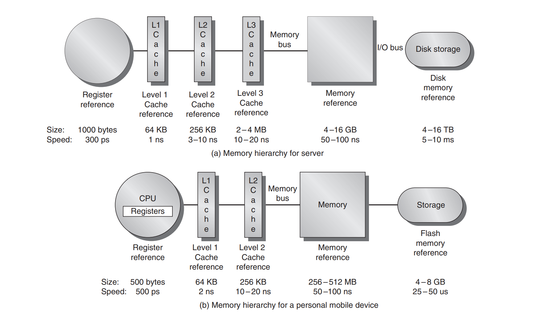
The concept of memory heirarchy came naturally as a result of the principle of locality. Not all data is accessed uniformly.

Memory Basics:

• Groups of adjacent memory are called blocks and theyre copied over to higher levels in the memory hierarchy for efficiency reasons (locality).
• Each block has a tag which maps to the memory address it corresponds to.
• Set associative is a design scheme on determining where in a cache to store blocks
• Sets are groups of blocks in a cache
• Blocks are mapped to a set by doing a (Block address) MOD (Number of sets in cache)
  • If there are n blocks in a set, the cache placement is called n-way set associative
  • If you have 1 block per set (a block is always placed in the same location), its called a direct-mapped cache
  • If you have just 1 set (a block can be placed anywhere), its called a fully associative cache
• Cache writing has some challenges like keeping copies of data in different levels of memory in sync while being written to
  • one strategy is write-through cache where you update both the item in cache and the one in main memory
  • another is a write-back cache where you only update the item in cache and when its about to be ejected from cache, it writes back the updated item to main memory
  • both strategies can use a write buffer
• Another important topic is cache-miss. This is when you search all levels of cache and you can’t find the memory you’re looking for. This is caused by three main reasons:
  • Compulsory: the data is just being accessed for the first time, so it hasn’t been written to cache yet
  • Capacity: the cache isn’t big enough to store all the blocks needed during execution of a program. When it fills up, it has to eject other blocks and those other blocks might need to be accessed
  • Conflict: If you have frequently accessed blocks that map to the same set, you get conflicts. Conflict misses occur when two (or more) memory blocks compete for the same spot (or set) in a cache. You can increase the associativity (decrease number of sets) to reduce this type of miss.

Appendix B

Cache is the name given to the highest or first level of the memory hierarchy encountered once the address leaves the processor

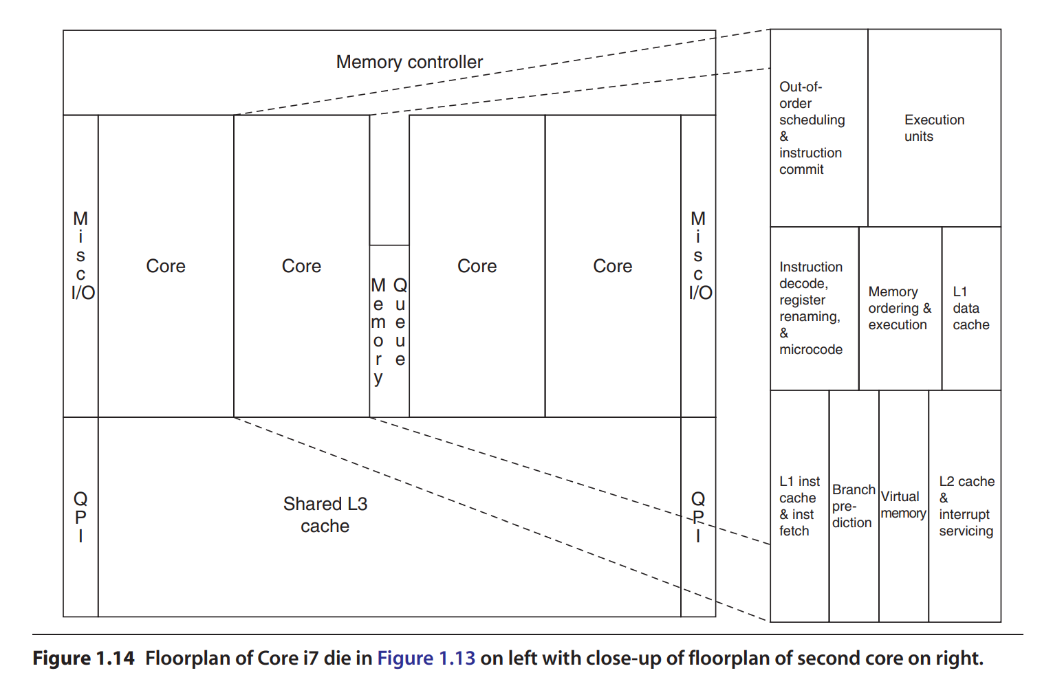
Physical CPU Layout V1

L3 cache being a part of the CPU depends on the CPU.

Word is a term used to describe the smallest unit of data the CPU requests from memory at one time. It would be 4 or 8 bytes if the CPU architecture were 32 bits or 64 bits accordingly.

Because of locality, we don’t just cache one word at a time, we bring blocks, or groups of words. Cache block size is fixed at the time of CPU design. It doesn’t dynamically change based on workload. The same goes to associativity (number of blocks per set)-that number is also fixed at hardware design time.

Virtual Memory

Virtual memory is a memory-management technique that gives programs the illusion that they have a very large, continuous address space—even larger than the actual physical RAM in the computer.

It does this by using both RAM (main memory) and disk storage (secondary storage), managing the placement and movement of data automatically and transparently.

Key Concepts of Virtual Memory:

1. Virtual vs. Physical Addresses:

   • Virtual Addresses: Used by programs; these addresses are logical and not directly mapped to physical memory.
   • Physical Addresses: Actual locations in RAM hardware.

   The system transparently translates virtual addresses into physical addresses via the Memory Management Unit (MMU).

2. Pages (Fixed-Size Blocks):

   • Virtual memory is divided into fixed-size blocks called pages (typically 4 KB or larger).
   • Similarly, physical memory is divided into blocks called frames of the same size.

   A page in virtual address space maps onto exactly one physical frame in RAM, or resides temporarily on disk.

3. Page Table:

   • A special data structure, the page table, maintains the mappings of virtual pages → physical frames.
   • It also indicates if a page is present in memory or currently stored on disk.

What’s a Page Fault?

When the CPU tries to access data on a page that’s not currently loaded in physical RAM (meaning it’s stored on disk), a page fault occurs.

Here’s how it works:

• CPU requests data at some virtual address.
• MMU checks the page table: the requested page isn’t in RAM (marked as “not present”).
• Page fault is triggered: OS software handles this situation by:
  1. Pausing the current task temporarily.
  2. Loading the requested page from disk into physical RAM.
  3. Updating the page table to reflect the new location of the page.
  4. Restarting the paused task.

Since disk access is much slower (milliseconds) than RAM access (nanoseconds), the processor doesn’t just wait—it usually switches to another task or thread while the page loads. When the page is finally ready, the original task resumes execution.

Project Ideas:

1. DRAM Access (row-conflict performance)
   • memory controller row hit priority performance